You're reading the documentation for a development version. For the latest released version, please have a look at v0.2.
Transient nutation: FFT
Classes used:
General description
Not all tr-EPR time traces show transient nutations, but if so, it may be of interest to extract the nutation frequency, as this allows to extract the local field strength of the microwave field at the sample location. The easiest way to extract the nutation frequency is by applying a 1D fast Fourier transform (FFT) along the time domain of the data.
The actual analysis step used, trepr.analysis.TransientNutationFFT, works with both, 1D and 2D datasets. The difference of the two scenarios shown below is more in the need for pre- and post-processing of the data.
Transient nutation analysis in 1D
In case of signals showing strong oscillations with the signal passing the zero line multiple times, there is usually no need for any pre-processing of the data, such as subtracting an exponential decay. Experimentally, this situation is typically found in crystalline samples of dilute paramagnetic species, such as a single crystal consisting of pentacene in a p-terphenyl matrix.
Recipe
 1format:
 2  type: ASpecD recipe
 3  version: '0.2'
 4
 5settings:
 6  default_package: trepr
 7  autosave_plots: false
 8
 9directories:
10  datasets_source: ../../tests/testdata/
11
12datasets:
13  - speksim/
14
15tasks:
16  - kind: processing
17    type: PretriggerOffsetCompensation
18    comment: >
19        Compensate for DC offsets of the signal prior to the laser flash
20  - kind: aspecd.processing
21    type: Averaging
22    properties:
23      parameters:
24        range: [370.4, 371.4]
25        unit: axis
26        axis: 0
27    result: 1Ddataset-averaged
28  - kind: singleplot
29    type: SinglePlotter1D
30    properties:
31      parameters:
32        tight: x
33        tight_layout: true
34    apply_to:
35      - 1Ddataset-averaged
36    result: time_trace
37  - kind: singleanalysis
38    type: TransientNutationFFT
39    properties:
40      parameters:
41        padding: 10
42    result: tnfft
43    comment: Perform FFT on dataset
44    apply_to: 1Ddataset-averaged
45  - kind: singleanalysis
46    type: TransientNutationFFT
47    properties:
48      parameters:
49        padding: 10
50        window: kaiser
51        window_parameters: [3]
52    result: tnfft-window
53    comment: Perform FFT on dataset
54    apply_to: 1Ddataset-averaged
55  - kind: multiplot
56    type: MultiPlotter1D
57    properties:
58      parameters:
59        tight_layout: true
60        show_legend: true
61      properties:
62        axes:
63          xlim: [0, 2e6]
64        drawings:
65          - label: no window
66          - label: Kaiser window
67        grid:
68          show: true
69          axis: x
70    result: fft
71    apply_to:
72      - tnfft
73      - tnfft-window
74  - kind: compositeplot
75    type: CompositePlotter
76    properties:
77      properties:
78        figure:
79          dpi: 150
80          size: [8, 4]
81      grid_dimensions: [1, 2]
82      subplot_locations:
83        - [0, 0, 1, 1]
84        - [0, 1, 1, 1]
85      plotter:
86        - time_trace
87        - fft
88      filename: transient-nutation-1d-fft.png
Result
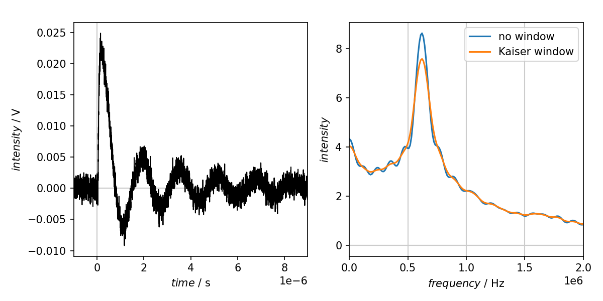
The resulting figure of the above recipe is shown below.

Result of the transient nutation analysis applying a 1D FFT along the time domain. The situation of no window and applying a Kaiser window is compared. For this case, no window would be necessary to extract the nutation frequency.
Transient nutation analysis in 2D
As mentioned above, the trepr.analysis.TransientNutationFFT analysis step does not care whether data are 1D or 2D, and can be applied to 2D data in the exact same way. The other difference here: The data used show still dominant transient nutations, but this time, the nutation is merely a modulation of the exponential decay. Hence, it is usually wise to subtract the exponential decay prior to applying the FFT.
Recipe
  1format:
  2  type: ASpecD recipe
  3  version: '0.2'
  4
  5settings:
  6  default_package: trepr
  7  autosave_plots: false
  8
  9directories:
 10  datasets_source: ../../tests/testdata/fsc2/
 11
 12datasets:
 13  #- radical-pair
 14  - triplet
 15
 16tasks:
 17  - kind: processing
 18    type: PretriggerOffsetCompensation
 19    comment: >
 20        Compensate for DC offsets of the signal prior to the laser flash
 21  - kind: processing
 22    type: BackgroundCorrection
 23    comment: >
 24        Correct for laser-induced background signal.
 25  - kind: singleanalysis
 26    type: TransientNutationFFT
 27    properties:
 28      parameters:
 29        padding: 10
 30        subtract_decay: True
 31    result: tnfft
 32    comment: Perform FFT on dataset
 33  - kind: singleanalysis
 34    type: TransientNutationFFT
 35    properties:
 36      parameters:
 37        padding: 10
 38        subtract_decay: True
 39        window: cosine
 40    result: tnfft-window
 41    comment: Perform FFT on dataset with cosine window
 42  - kind: singleanalysis
 43    type: BasicCharacteristics
 44    properties:
 45      parameters:
 46        kind: max
 47        output: indices
 48        axis: 0
 49    result: max_field
 50  - kind: processing
 51    type: SliceExtraction
 52    properties:
 53      parameters:
 54        position: max_field
 55        axis: 0
 56    result: time_trace_max
 57    comment: Extract transient for global maximum of the dataset
 58  - kind: singleanalysis
 59    type: BasicCharacteristics
 60    properties:
 61      parameters:
 62        kind: min
 63        output: indices
 64        axis: 0
 65    result: min_field
 66  - kind: processing
 67    type: SliceExtraction
 68    properties:
 69      parameters:
 70        position: min_field
 71        axis: 0
 72    result: time_trace_min
 73    comment: Extract transient for global minimum of the dataset
 74  - kind: processing
 75    type: SliceExtraction
 76    properties:
 77      parameters:
 78        position: max_field
 79        axis: 0
 80    result: frequency_max
 81    comment: Extract frequency for global maximum of the dataset
 82    apply_to: tnfft
 83  - kind: processing
 84    type: SliceExtraction
 85    properties:
 86      parameters:
 87        position: min_field
 88        axis: 0
 89    result: frequency_min
 90    comment: Extract frequency for global minimum of the dataset
 91    apply_to: tnfft
 92  - kind: processing
 93    type: SliceExtraction
 94    properties:
 95      parameters:
 96        position: max_field
 97        axis: 0
 98    result: frequency_max-window
 99    comment: Extract frequency for global maximum of the dataset
100    apply_to: tnfft-window
101  - kind: processing
102    type: SliceExtraction
103    properties:
104      parameters:
105        position: min_field
106        axis: 0
107    result: frequency_min-window
108    comment: Extract frequency for global minimum of the dataset
109    apply_to: tnfft-window
110  - kind: singleplot
111    type: SinglePlotter2D
112    properties:
113      parameters:
114        tight_layout: true
115      properties:
116        figure:
117          dpi: 300
118      type: contourf
119    result: original_data
120  - kind: singleplot
121    type: SinglePlotter2D
122    properties:
123      parameters:
124        tight_layout: true
125      properties:
126        figure:
127          dpi: 300
128        axes:
129          ylim: [0, 8e5]
130      type: contourf
131    result: fft_data
132    apply_to: tnfft-window
133  - kind: multiplot
134    type: MultiPlotter1D
135    properties:
136      parameters:
137        tight_layout: true
138        tight: x
139      properties:
140        grid:
141          show: true
142          axis: x
143    result: time_traces
144    apply_to:
145      - time_trace_max
146      - time_trace_min
147  - kind: multiplot
148    type: MultiPlotter1D
149    properties:
150      parameters:
151        tight_layout: true
152        show_legend: true
153      properties:
154        axes:
155          xlim: [0, 5e5]
156        drawings:
157          - label: max
158          - label: min
159          - label: max cosine
160          - label: min cosine
161        grid:
162          show: true
163          axis: x
164    result: frequency_traces_compare_windows
165    apply_to:
166      - frequency_max
167      - frequency_min
168      - frequency_max-window
169      - frequency_min-window
170  - kind: multiplot
171    type: MultiPlotter1D
172    properties:
173      parameters:
174        tight_layout: true
175      properties:
176        axes:
177          xlim: [0, 5e5]
178        grid:
179          show: true
180          axis: x
181    result: frequency_traces
182    apply_to:
183      - frequency_max-window
184      - frequency_min-window
185  - kind: compositeplot
186    type: CompositePlotter
187    properties:
188      properties:
189        figure:
190          dpi: 150
191          size: [8, 7]
192      grid_dimensions: [2, 2]
193      subplot_locations:
194        - [0, 0, 1, 1]
195        - [0, 1, 1, 1]
196        - [1, 0, 1, 1]
197        - [1, 1, 1, 1]
198      plotter:
199        - original_data
200        - fft_data
201        - time_traces
202        - frequency_traces
203      filename: transient-nutation-2d-fft.png
Result
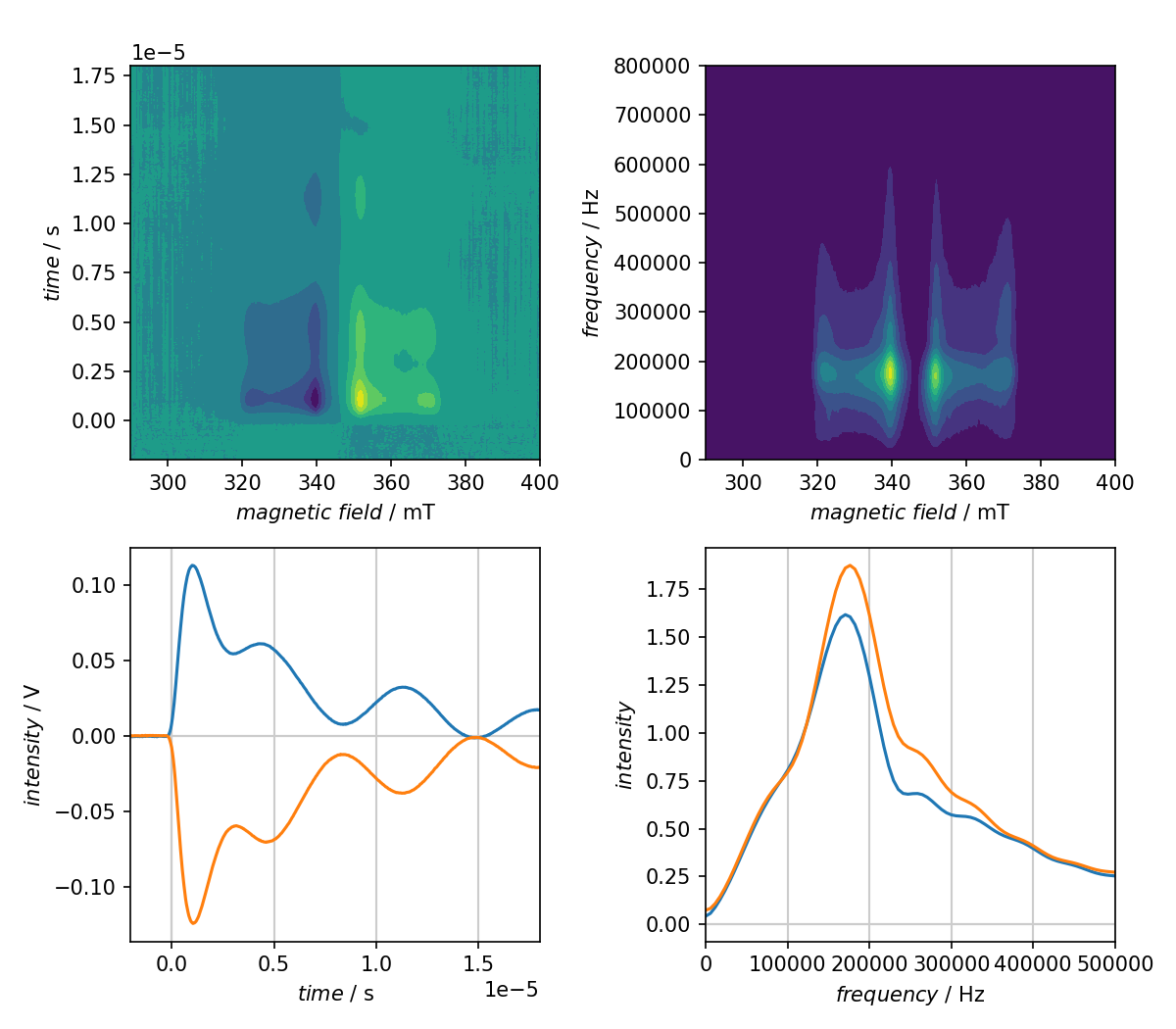
The resulting figure of the above recipe is shown below.

Result of the transient nutation analysis of a full 2D dataset by applying a 1D FFT along the time domain. The transient nutation frequencies for the absorptive and emissive signal maxima are shown.