You're reading the documentation for a development version. For the latest released version, please have a look at v0.2.
Time taken per individual time trace
Classes used:
General description
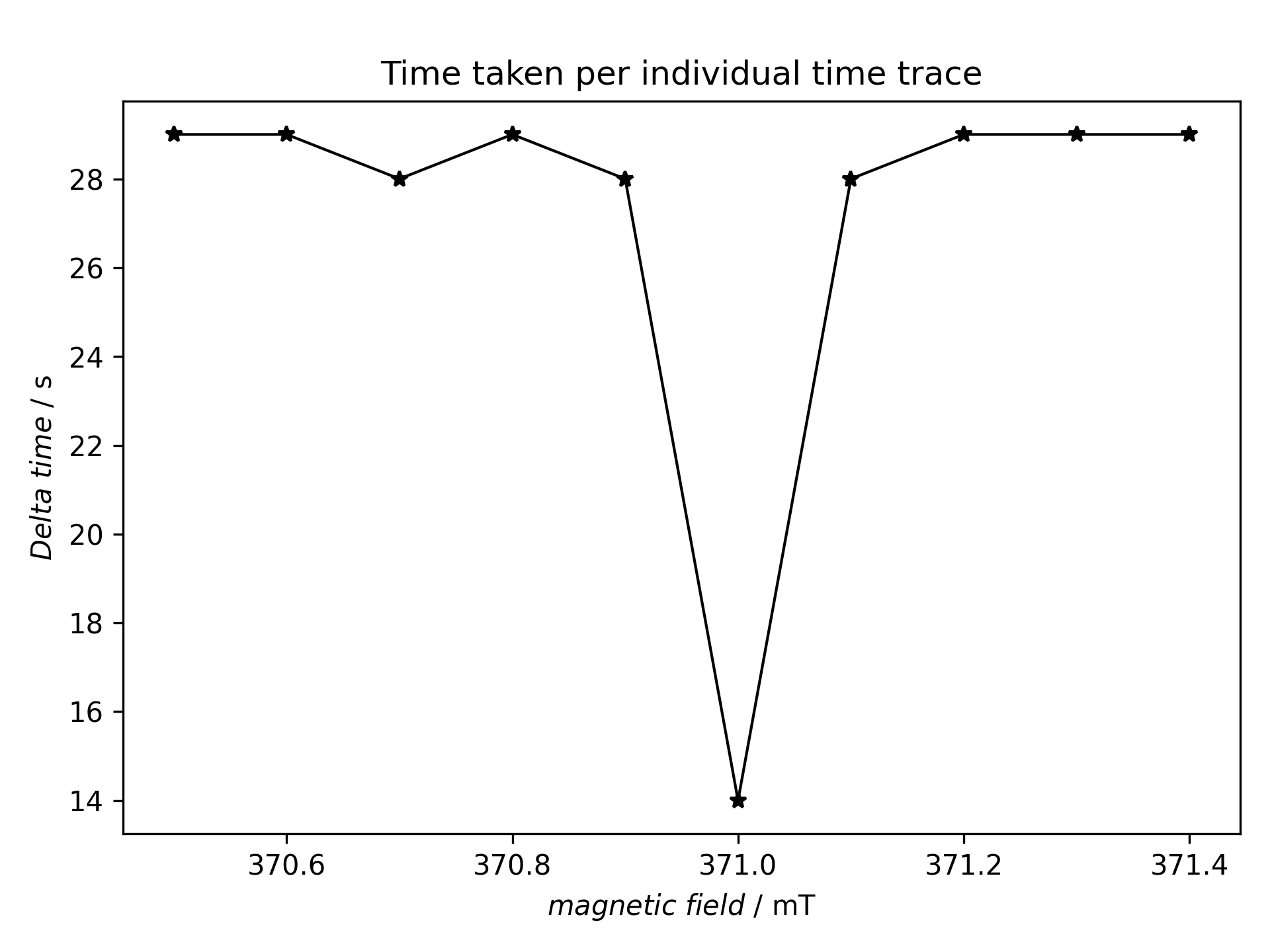
tr-EPR experiments usually take quite some time (hours rather than minutes) due to their 2D character. Generally, the time taken per time trace should be the same on average. Hence, it is a good way to check whether everything went well to simply plot the time taken per individual time trace as a function of the magnetic field positions. If there are some dramatic deviations, this is a good hint of some (intermediate) problems.
A necessary prerequisite to figure out how long recording of each individual time trace took is to record time stamps during the measurement, one per time trace. Using a commercial Bruker setup and software, this is usually not (easily) possible. However, if you use some lab-built software to control your tr-EPR setup, it is entirely up to this software.
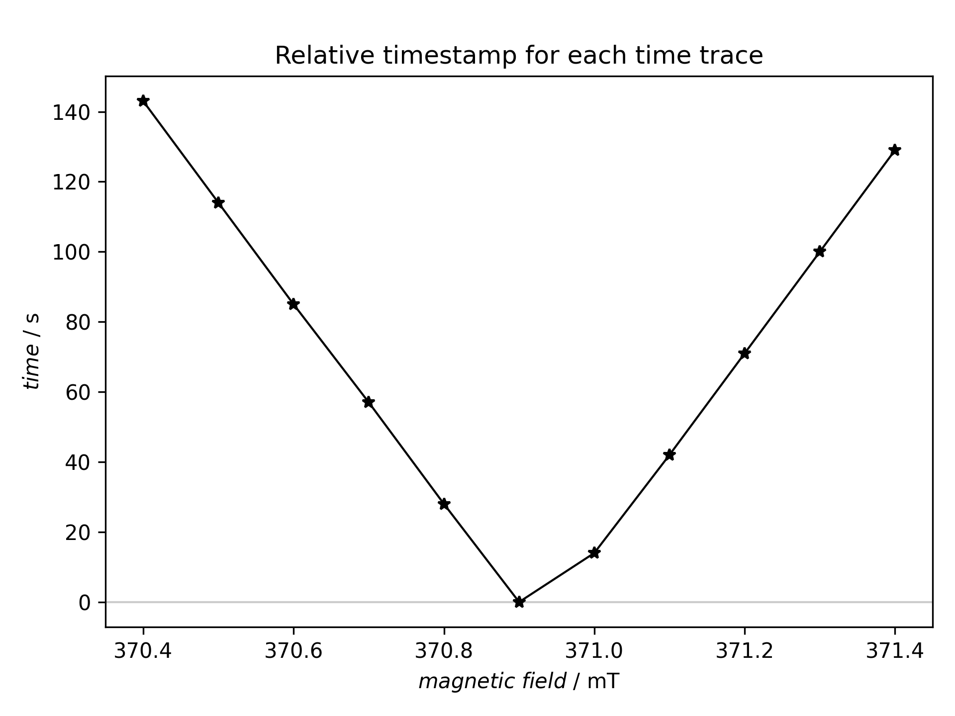
The following example demonstrates what is possible when the relevant information is available for each individual time trace. Basically, the recipe creates two plots: the relative time (starting with the start of the measurement) each of the time traces has been recorded as function of the magnetic field, and the difference in time taken between two time traces as function of the magnetic field.
Recipe
 1format:
 2  type: ASpecD recipe
 3  version: '0.2'
 4
 5settings:
 6  default_package: trepr
 7
 8directories:
 9  datasets_source: ../../tests/testdata/
10
11datasets:
12- speksim/
13
14tasks:
15- kind: singleanalysis
16  type: TimeStampAnalysis
17  properties:
18    parameters:
19      kind: delta
20      output: dataset
21  result: time-delta
22- kind: singleplot
23  type: SinglePlotter1D
24  properties:
25    parameters:
26      tight_layout: true
27    properties:
28      drawing:
29        marker: '*'
30      figure:
31        dpi: 300
32      axes:
33        title: Time taken per individual time trace
34    filename: time-delta.png
35  apply_to: time-delta
36- kind: singleanalysis
37  type: TimeStampAnalysis
38  properties:
39    parameters:
40      kind: time
41      output: dataset
42  result: time-values
43- kind: singleplot
44  type: SinglePlotter1D
45  properties:
46    parameters:
47      tight_layout: true
48    properties:
49      drawing:
50        marker: '*'
51      figure:
52        dpi: 300
53      axes:
54        title: Relative timestamp for each time trace
55    filename: time-values.png
56  apply_to: time-values
Result
The recipe actually creates two figures presented afterwards.

The position in time (relative time stamp) for each individual time trace. The perhaps unexpected shape results from the fact that the data have not been recorded from low to high field (or vice versa), but inside out, starting at the centre position of the magnetic field axis.

Relative time taken for each individual time trace. The perhaps unexpected shape results from the fact that the data have not been recorded from low to high field (or vice versa), but inside out, starting at the centre position of the magnetic field axis. This is why the difference between the first and second recorded time trace is half of the difference between all other time traces.